Denoising binary images |

Data science is transforming the world: we already see self-driving cars moving from research to production, data-driven cancer diagnostic systems, machine learning trader bots and lots of other exciting technologies because the corresponding problems have been reduced to understanding data. While the science of data for centuries was known as statistics, computer scientists, together with other scientists like physicists have given a new meaning to the term data science. Currently data science is an interdisciplinary field that uses tools from various fields to extract knowledge and insights from data in various forms. What follows is an introductory example that I use in my data science class at Boston University to illustrate some aspects of solving a data science problem. The problem is how to denoise images. We are given a noisy version of an image and we wish to denoise it, namely recover the content behind it. Clearly, this is an ill-defined problem: since what we observe is a noisy version of some signal, in theory that signal could be anything. This is really common in data science problems: we need to make some reasonable assumptions about our problem. I will use Python to write code in order to show you a fairly complete view of the problem.

Denoising images

Let’s start by writing the letter T using numpy in Python, encoded in a 0/1 array.

image_t = np.array(
 [[ 0, 0, 0, 0, 0, 0, 0, 0, 0, 0, 0, 0, 0,],
 [ 0, 0, 0, 0, 0, 0, 0, 0, 0, 0, 0, 0, 0,],
 [ 0, 0, 1, 1, 1, 1, 1, 1, 1, 1, 1, 0, 0,],
 [ 0, 0, 1, 1, 1, 1, 1, 1, 1, 1, 1, 0, 0,],
 [ 0, 0, 1, 1, 1, 1, 1, 1, 1, 1, 1, 0, 0,],
 [ 0, 0, 0, 0, 0, 1, 1, 1, 0, 0, 0, 0, 0,],
 [ 0, 0, 0, 0, 0, 1, 1, 1, 0, 0, 0, 0, 0,],
 [ 0, 0, 0, 0, 0, 1, 1, 1, 0, 0, 0, 0, 0,],
 [ 0, 0, 0, 0, 0, 1, 1, 1, 0, 0, 0, 0, 0,],
 [ 0, 0, 0, 0, 0, 1, 1, 1, 0, 0, 0, 0, 0,],
 [ 0, 0, 0, 0, 0, 1, 1, 1, 0, 0, 0, 0, 0,],
 [ 0, 0, 0, 0, 0, 1, 1, 1, 0, 0, 0, 0, 0,],
 [ 0, 0, 0, 0, 0, 1, 1, 1, 0, 0, 0, 0, 0,],
 [ 0, 0, 0, 0, 0, 1, 1, 1, 0, 0, 0, 0, 0,],
 [ 0, 0, 0, 0, 0, 0, 0, 0, 0, 0, 0, 0, 0,],
 [ 0, 0, 0, 0, 0, 0, 0, 0, 0, 0, 0, 0, 0,]])

Let’s visualize this.

import matplotlib.pyplot as plt
import matplotlib.cm as cm
%matplotlib inline

plt.imshow(image_t,cmap=cm.gray)
plt.axis('off')

This is what we get, indeed the array represents the letter “T”.

Now, let’s generate a corrupted version of this image by flipping each bit with some probability p. We can also do it a bit faster using utilities of numpy (corrupt_image_fast)

import random
def corrupt_image(image,p=0.15):
corrupted = image.copy()
    rows, cols = corrupted.shape
    for r in range(rows):
        for c in range(cols):
            if random.random() &lt;= p :
                corrupted[r][c] = 1 - corrupted[r][c] #flip pixel
    return corrupted

def corrupt_image_fast(image,p=0.15):
corrupted = image.copy()
rows, cols = corrupted.shape
prob = np.random.rand(rows,cols)
corrupted = np.multiply(corrupted, prob&gt;p) + np.multiply(1-corrupted, prob&lt;=p)
return corrupted

Let’s range the corruption probability from 0 to 1 with a step of 0.05 and see what we get.

plt.figure(1)
index = 1
for p in np.linspace(0,1,21):
    plt.subplot(3,7,index)
    plt.title(repr("{:1.2f}".format(p)))
    plt.imshow( corrupt_image_fast(image_t,p), cmap=cm.gray)
    plt.axis('off')
    index+=1

Noisy version of the original image.

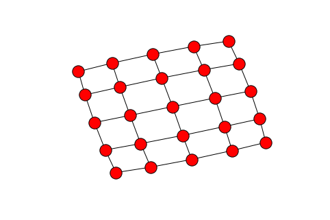
Therefore our problem informally is how can we get from the noisy image in the right to the original image? What are the modelling assumptions that we can use that would make the original image most likely? Think about other letters or digits. They are structured. The image consists of homogeneous patches that suddenly change when we get close to the boundaries. We impose the natural grid structure on the image, where each node corresponds to a pixel, and edges to neighboring pixels corresponding to the four possible directions, north, south, west, east. Here is a visualization of a $5\times 5$ grid. grid

Modelling: Each node $i$ on the grid has a binary value $x_i \in \{0,1\}$ , corresponding to whether the pixel is on or off in the image. We will model the recovery problem probabilistically. Let us assume that what we observe is the signal $y=(y_1,\ldots,y_n)$ and the original image is the signal $x=(x_1,\ldots,x_n)$ . We will maximize the conditional probability $p(x|y)$ over all possible original signals $x$ . We impose our intuitive assumptions we discussed above by imposing an appropriate prior probability distribution on $x$ . Specifically, we assume that the probability of $x$ is proportional to $\exp\Big( \frac{1}{2} \sum_{i \neq j} \beta_{ij} (x_i x_j +(1-x_i)(1-x_j) \Big)$ . Why is this a good prior? For any edge between two pixels $i,j$ with the same value the exponent is equal to $\frac{1}{2}(x_i^2+(1-x_i)^2)=\frac{1}{2}$ . On the contrary, when the pixel values differ the exponent is equal to $0$ . Hence the prior encourages homogeneous patches. This is known as a locally dependent Markov Random Field (MRF). We use Bayes’ rule to compute the conditional probability $p(x|y)$ we care about. $p(x|y) \propto p(x) p(y|x)$ . First we compute the likelihood function $p(y|x)$ . Let $f(y_i|x_i)$ be the conditional density function for all $i \in [n]$ . For the sake of our exposition we have assumed in this lecture $f(1|1)=f(0|0)=1-p, f(0|1)=f(1|0)=p$ . We will assume that the pixel noise is iid. Notice that there are real cases where the noise is localized and forms “patches” too. The iid assumption simplifies a lot the computation of the likelihood function as it factors over the pixels, namely $p(y|x) = \prod_{i=1}^n f(y_i|1)^{x_i}f(y_i|0)^{1-x_i}$ . According to Bayes’ rule $p(x|y) = \frac{p(y|x)p(x)}{p(y)}$ . Maximizing $p(x)$ is equivalent to maximizing the nominator as the denominator does not depend on $x$ . This is convenient computationally as computing the marginal distribution $p(y)$ is not easy, at least the straightforward computation $p(y) = \sum_x p(y|x) p(x)$ requires summing over $2^n$ possible values of $x$ . Equivalently, due to the monotonicity of the $log$ function we can try to maximize $\log{p(x|y)}= \log{p(y|x)}+\log{p(x)}$ .

$\begin{aligned} \log{p(x|y)} &= \frac{1}{2} \sum_{i,j} \beta_{ij}\big( (1-x_i)(1-x_j)+x_ix_j \big) + \sum_{i=1}^n \big(x_i \log{f(y_i|1)} +(1-x_i) \log{f(y_i|0)} \big) \\ &=\frac{1}{2} \sum_{i,j} \beta_{ij}\big( (1-x_i)(1-x_j)+x_ix_j \big) + \sum_{i=1}^n x_i \log{\frac{f(y_i|1)}{f(y_i|0)}} +\sum_{i=1}^n \log{f(y_i|0)}. \end{aligned}$

The last term does not depend on our variable $x$ , so our problem is to maximize the objective

$\begin{aligned} L(x|y) &=\sum_{i=1}^n \lambda_i x_i + \frac{1}{2} \sum_{i,j} \beta_{ij}\big( (1-x_i)(1-x_j)+x_ix_j \big), \end{aligned}$

where $\lambda_i =\log{\frac{f(y_i|1)}{f(y_i|0)}}$ . Observe that $\lambda_i$ may also take negative values. For example, suppose $p=0.15$ . According to the probabilistic model we coded up in Python, if $y_i=1$ , $\lambda_i=\log{\frac{0.8}{0.2}}=\log 4>0$ . However, if $y_i=0$ , $\lambda_i=-\log 4<0$ . Now we will refresh our combinatorial optimization toolbox. We are optimizing over discrete signals $x$ , and there are $2^n$ possible such signals since for each pixel there are two possible values. Observe that since $x_i \in \{0,1\}, x_i=x_i^2$ , and therefore $(1-x_i)(1-x_j)+x_ix_j=1+2x_ix_j -x_i -x_j = 1- (x_i^2+x_j^2-2x_ix_j) =1-(x_i-x_j)^2$ . This suggests that the second term has to do with a cut function since $(x_i-x_j)^2$ is 1 if the edge $(i,j)$ connects endpoints with different pixel values. It turns out that indeed our maximization problem can be reduced to a minimum cut/maximum flow computation. Specifically, we create a network as follows.

We create two extra nodes, the source and the sink $s,t$ respectively.
We add an arc from the source $s$ to each node $i$ for which $\lambda_i>0$ . We set the capacity to be $\lambda_i$.
We add an arc from each node $i$ for which $\lambda_i\leq 0$ to the sink $t$. We set the capacity to be $-\lambda_i$.
For each pair of neighboring nodes $\{i,j\}$ , we add two directed edges $(i,j),(j,i)$ with capacity $\beta_{ij}$ .

For any binary image $x=(x_1,\ldots,x_n)$ let $S=s \cup \{i:x_i=1\}$ , and $T=t \cup \{i:x_i=0\}$ . The cut value is equal to

$\begin{aligned} C(x) &= \sum_{i=1}^n x_i \max(0,-\lambda_i) + \sum_{i=1}^n (1-x_i) \max(0,\lambda_i) + \frac{1}{2} \sum_{i,j} \beta_{ij} (x_i-x_j)^2. \end{aligned}$

This is precisely our objective negated shifted by a constant. Hence, minimize this cut value is equivalent to our maximization problem. We can solve this using max flows in polynomial time! Here is an alternative view of our objective. We are given a binary matrix that is associated with a cost proportional to the number of edges of the corresponding grid that connect endpoints with different values (call such edges bad). We are allowed to flip an entry of the binary matrix if we pay $K$ dollars (i.e., per entry we change). For each bad edge we pay $R$ dollars.Hence the total cost of our choice is equal to

$\begin{aligned} \text{Cost of our choice}&=K \times \#(\text{entries we flip}) +R\times \#(\text{bad edges}). \end{aligned}$

This of course corresponds to a special case of the weights $\lambda_i, \beta_{ij}$ but captures fully our problem. Let’s see how we can translate all the above into Python code. We will use igraph, a useful package for graph algorithms in Python (another useful one is networkx) and for simplicity we will assume $\beta_{ij}=\alpha$ for all neighboring $i,j$ . Also let $\beta=|\lambda_i|$ according to our simple choice of a conditional density function. Let’s assume that $p<0.5$ , therefore since $1-p>p$ we get that $\lambda_i > 0$ for all pixels such that $y_i=1$ .

def create_graph(img, K=1, lambda=3<span id="mce_SELREST_start" style="overflow:hidden;line-height:0;"></span>.5):
     max_num = len(img)*len(img[0])
     s,t = max_num, max_num + 1
     edge_list = []
     weights = []
     for r_idx, row in enumerate(img):
         for idx, pixel in enumerate(row):
                  px_id = (r_idx*len(row)) + idx
                  #add edge to cell to the left
                  if px_id!= 0:
                      edge_list.append((px_id -1, px_id))
                      weights.append( K )
                   #add edge to cell to the right
                   if px_id != len(row) -1:
                       edge_list.append((px_id +1, px_id))
                       weights.append( K )
                   #add edge to cell to the above
                   if r_idx!= 0:
                       edge_list.append((px_id - len(row), px_id))
                       weights.append( K )
                    #add edge to cell to the below
                    if r_idx != len(img) -1:
                       edge_list.append((px_id + len(row), px_id))
                       weights.append( K )
                    #add an edge to either s (source) or t (sink)
                   if pixel == 1:
                      edge_list.append((s,px_id))
                      weights.append( lambda )
                   else:
                      edge_list.append((px_id, t))
                      weights.append( lambda )
          return edge_list, weights, s, t

Now we can run max flow on this network to get our min cut as follows.

def recover(noisy, K=1, lambda=3.5):
        edge_list, weights, s, t = create_graph(noisy, K,lambda)
        g = igraph.Graph(edge_list)
        output = g.maxflow(s, t, weights)
        recovered = np.array(output.membership[:-2]).reshape(noisy.shape)
        return recovered

plt.imshow(recover(corrupt_image_fast(image_t,0.15), 1, 3.5))

For $K=1, \lambda=3.5$ we obtain the following recovery result for our image representing letter T.

recovery

For more, check out the following references:
[1] Lecture 1, Data Analytics class
[2] Exact Maximum a Posteriori inference for binary images

Preliminaries

For those not familiar with Bayes’ rule and flows in networks, the Wikipedia articles are a good start.

Denoising binary images

Denoising images

Preliminaries

Leave a Reply Cancel reply

Follow webpage via email

Denoising binary images

Denoising images

Preliminaries

Share this:

Like this:

Leave a Reply Cancel reply

Follow webpage via email